Dmitry A. Kazakov
(mailbox@dmitry-kazakov.de)
ON INTUITIONISTIC FUZZY MACHINE LEARNING
Dmitry A. Kazakov
(mailbox@dmitry-kazakov.de)
![]()
© 2005 Dmitry A. Kazakov
Abstract: The aim of this work is to propose an intuitionistic formulation of the machine learning problem, completely independent from probability theory. Intuitionistic fuzzy sets naturally appear in machine learning based on possibility theory as a result of uncertainty in the measuring process. Considering this only type of uncertainty, a notion of fuzzy feature as a mapping can be defined. Fuzzy features originate four different pattern spaces. Fuzzy classification is defined as a pair of images in the pattern spaces. Properties of the fuzzy pattern spaces required for fuzzy inference are demonstrated.
1. Introduction
2. Fuzzy events, features, classes
2.1 Fuzzy features
2.2 Fuzzy images
2.3 Multiple features, independent features
2.4 Fuzzy classes and classifiers
3. Learning
4. Properties of pattern space
5. Final notes
6. Selected bibliography
7. Proofs
The concept of learning (training) and classification is based on the notion of feature. A feature is something that can be measured and then used for classification. I assume that the process of measurement cannot be separated from what is being measured. In other words the measured thing cannot be sensed directly. This is how uncertainty usually comes into play. Whether this uncertainty is a part of the "real world" or a side effect of the measurement process is only of philosophical interest. We could observe two different kinds of uncertainty: randomness and fuzziness. A statistical or probabilistic approach to pattern recognition[Tou74] treats whole uncertainty as randomness. With this approach the features become random variables. On contrary a fuzzy approach treats uncertainty as fuzziness, so the fuzzy features become mappings resulting in fuzzy subsets[Zad65] of the feature domain set.
It is important to note that neither probabilistic nor fuzzy approach may supersede another, because neither randomness nor fuzziness can be adequately described by another. So it would be wrong to think of the fuzzy pattern recognition theory as a generalization of the statistical one Neither it is an alternative theory, because they have different, though intersecting, application domains. There well could be also intermixed variants of both. It is also important to observe that the features related to physical processes would most likely be random variables. For instance, the quantum mechanics is based solely on the probability theory. One could ask, why not to always use the statistical approach for physical processes? The answer is, yes, do it when it works. Unfortunately, in many cases it does not. And even if the "real word" is not the source of fuzziness, but the way we perceive it definitely is. So the theories we invent to describe it are. Often the fuzzy component in our knowledge of a physical process prevails any uncertainty the randomness of the process may contribute. I.e. we know so little that it makes no difference. The bottom line is, only if deterministic methods do not work, if statistical models are inadequate, then one should choose fuzzy methods.
In this work I formulate the problem of fuzzy learning and explain the basics of the chosen approach, being as informal and short as possible. I hope that a careful reader will be able to fill missing details. This work continues my PhD thesis[Kaz92] and later works[Gep93], but on a more solid ground. Earlier works were rather empirical, though the understanding of importance of upper and lower sets was clear already then. Now, as I hope, it is obvious that from intuitionistic point of view fuzzy mappings should induce two more images. All four induced pattern spaces can be used for learning. Another difference is settled understanding that fuzzy approach needs no props of the probability theory.
Space of elementary events Ω is a set of some elements ω∈Ω, only known that they exist and are mutually independent (do not intersect). A fuzzy event p is defined as a fuzzy subset of Ω, i.e. p:Ω→[0,1]. There is little sense to distinguish fuzzy sets from their membership functions. Everywhere below they will be considered same. The value p(ω) tells how possible is that ω belongs to p. It is also noted as Pp|{ω}. For different elementary events do not intersect, the necessity that ω belongs to p: Np|{ω} = 1 - Pp|{ω} is also p(ω). Fuzzy events do not necessarily happen as random events do, however they could. Anyway we will not define any additive measure on Ω and thus will not assume that ω have any probability.
Conditional possibility [Dub88] of a fuzzy event p provided another fuzzy event q is:
Pp|q = Sup
ω∈Ωmin (p(ω), q(ω)) = Sup
ω∈Ωp(ω)&q(ω) = Pp∩q
Conditional necessity [Dub88] of p provided q is Np|q = 1 - Pp|q:
Np|q = Inf
ω∈Ωmax (p(ω), 1 - q(ω)) = Inf
ω∈Ωp(ω)∨q(ω) = Np∪q
A possibility-necessity pair (Pp|q, Np|q) tells us how possible and necessary is that q is a subset of p. For an elementary event ω we have Pp|{ω} = Np|{ω} = p(ω). This is why the elementary events are called so. To know either the possibility or necessity is all that one needs. Usually the elementary events are unavailable for direct perception. It means that for a given event p there is no way to obtain the membership function p(ω). The only thing known about p is its properties, or else features which can be measured on it. For instance, we cannot directly perceive a man. Instead of that we could measure his height, sense the color of his eyes, learn the features of his face, etc.
From the point of view of intuitionistic fuzzy set theory[Ata98], the pair (Pp|q, Np|q) can be viewed as a intuitionistic fuzzy proposition that q⊆p. In this proposition μq⊆p = Pp|q, γq⊆p = 1 − Np|q. The intuitionistic fuzzy approach combines four-valued logic of Dunn and Belnap[Bel77] with Zadeh's generalization of truth values. It is characteristic for intuitionistic approach to consider truth and falsehood being relative[Shra00]. The pair can also be viewed as an interval because necessity is normally lower than possibility.
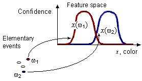
Fuzzy feature x with the domain set Dx[Kaz92] is a measurable function that for each elementary event ω∈Ω and each domain value d∈Dx gives us the possibility that x obtains the value d when ω is observed: x:Ω×Dx→[0,1]. Let we fix some elementary event ω, then x(ω,·) can be viewed as a fuzzy subset of Dx. This subset we will denote as x(ω) and call the image of ω in the pattern space of x. If we fix some feature value d, then x(·,d)=x(d) being viewed as a fuzzy subset of Ω, is the original of d in Ω.
Pattern space of a feature x is the set of all possible fuzzy subsets of the domain set of x, i.e. [0,1]Dx. Images of different elementary events may intersect in the pattern space as shown on the picture:
The features should be normal. The normality of a feature means that both x(ω,·) and x(·,d) are normal fuzzy sets for any ω and d, i.e.
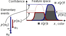
So far we have had only images of the elementary events and the originals of the feature domain values. The next step is to define images of any fuzzy event. We can do it because x is a measurable function. Consider a fuzzy event p:Ω→[0,1]. It has two images in the pattern space of x defined as follows: ∀d∈Dx
x(p)↑(d) = Sup
ω∈Ωx(ω,d) & p(ω) = Px(d)|p = Px(d)∩p x(p)↓(d) = Inf
ω∈Ωx(ω,d) ∨ p(ω) = Nx(d)|p = Nx(d)∪p = 1-Px(d)|p
In general case these images are different. They are same for the elementary events: x(ω)=x({ω})↑=x({ω})↓. The following picture illustrates the formulae for the images. Here p consists of the elementary events ω1 and ω2 with the possibilities of p(ω1) and p(ω2) correspondingly:
Informally, a fuzzy feature is some value being measured. For instance let hair color be a feature to classify persons. Then Dcolor is the set of colors: {blond, red,...}. A classification of someone's hair color is a set of fuzzy logical values telling whether the person is blond (belongs to the set of blond persons), red etc. This classification is comprised of images in the space of hair colors. Normality of the feature hair color means that for any color of hair there is at least one persons having it and that any person has hair of some color.
For a fuzzy event p we could also have images of the complement event p. Which gives us the four fundamental characteristics of p:
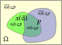 |
Px(d)⊆p | = | x(p)↑(d) | = | Pp⊆x(d) | p has x(d) in | ||
| Px(d)⊆p | = | x(p)↑(d) | = | 1-Nx(d)⊆p | p has x(d) outside | |||
| Px(d)⊆p | = | 1 - x(p)↓(d) | = | 1-Np⊆x(d) | p has not-x(d) | |||
| Px(d)⊆p | = | 1 - x(p)↓(d) | p has not-x(d) outside |
The most important objects obtained from these four characteristics are fuzzy estimation and fuzzy classification of an event in the pattern space.
Fuzzy estimation of p in the pattern space of x we define as the pair of images:
p[x] = ( x(p)↑, ) has-in, has-out
It is a proper intuitionistic set, which upper set p[x]↑ is x(p)↑ and the lower set p[x]↓ is inversed x(p)↑. p[x] estimates p in the pattern space of x. Values of the membership functions of the upper and lower sets in some d, combined in a fuzzy logical value
( p[x]↑(d), p[x]↓(d) )
characterize x(d)⊆p. These logical values are consistent because p[x]↑ dominates p[x]↓, i.e.
∀d∈Dx p[x]↑ ≥ p[x]↓(d) (2.2.1)
An important result about fuzzy estimations is that, if known, we can judge whether q is a fuzzy subset of p:
Pp[x]↑|q[x]↑ = Pp[x]↑∩q[x]↑ ≥ Pp|q (2.2.2) Np[x]↓|q[x]↑ = Np[x]↓∪q[x]↑ ≤ Np|q (2.2.3)
Fuzzy classification is defined as the pair of images:
x(p) = ( x(p)↑, x(p)↓ ) has-in, has-not
The values of the membership functions of the upper set and the lower set combined in a fuzzy logical value:
( x(p)↑(d), x(p)↓(d) )
tell us how possible and necessary is that p⊆x(d). So they classify p into of the domain set of the feature x. x(p) is an intuitionistic classification. The for any normal p x(p)↑ dominates x(p)↓:
∀d∈Dx x(p)↑(d) ≥ x(p)↓(d) (2.2.4)
Which of the four characteristics are available during learning and classification depends on the concrete application. Usually measured values are classifications, while expert knowledge is represented in terms of estimations (proper intuitionistic sets). In a real system one can have both classifications and estimations mixed. For example, when the measured data are combined with a priory known facts. The following table summarizes the relationship between estimations and classifications for a fuzzy event p and a feature x:
p[x]↑ = x(p)↑ = = - has-in = x(p)↑ = p[x]↑ = - has-out p[x]↑ = = = x(p)↑ - has-not = = p[x]↑ = x(p)↑ - has-not-out
Let x be a vector feature with N coordinates from the domain sets Di=1..N:
x(ω,d) = x(ω, d1 ) = x(ω,d1,d2,...,dN)∈[0,1] d2 ... dN
The domain set of x is a Cartesian product of the component's domain sets. The sets Di are often considered as the domain sets of some partial features xi corresponding to the coordinates and defined as projections:
xi(ω,t) = Sup x(ω,d)
d∈Dx|di=t
It is said that features xi are independent if their joint distribution x(ω,d1,d2,...,dN) can be split into projections:
x(ω,d1,d2,...,dN) = Min
i=1..Nxi(ω,di):
Unlikely to the probability theory, even if features xi are not independent one can always estimate their joint distribution:
x(ω,d1,d2,...,dN) ≤ Min
i=1..Nxi(ω,di)
Images of an event p can be estimated using its projections:
x(p)↑(d) ≤ Min
i=1..Nxi(p)↑(di) (2.2.5) x(p)↓(d) ≥ Max
i=1..Nxi(p)↓(di) (2.2.6)
So the estimations (2.2.2) and (2.2.3) for many features take form:
Min
i=1..NPp[xi]↑|q[xi]↑ ≥ Pp|q (2.2.7) Max
i=1..NNp[xi]↓|q[xi]↑ ≤ Np|q (2.2.8)
Also for complement feature projections xi (under definite conditions):
Max
i=1..NPp[xi]↑|q[xi]↑ ≥ Pp|q (2.2.9) Min
i=1..NNp[xi]↓|q[xi]↑ ≤ Np|q (2.2.10)
Fuzzy classes are naturally represented by some dedicated fuzzy events. Let C be a set of fuzzy classes C={cj | cj:Ω→[0,1]}, then it induces a fuzzy feature, so-called class-feature c:Ω×C→[0,1], defined as c(ω, cj)=cj(ω). The domain set of the class-feature is the set of classes. Then for a fuzzy class cj a fuzzy classification of p into the domain set of the class-feature c is
c(p)↑(cj) = Pcj|p
c(p)↓(cj) = Ncj|p
i.e. the possibility and necessity that p⊆cj. Observe a direct analogy to the Bayesian classifiers.
Fuzzy classifier is a function that for images of an event p yields an estimation of the fuzzy classification of p, such that for the class cj Pcj|p is estimated from above, Ncj|p is from below.
Learning is a process of building and tuning a classifier. In order to do it one could try to build images of the classes cj and their complements cj in the pattern space. Having these two images we could classify an event p by measuring the distances from the image of p to the images of cj and cj. This method of classification is called minimum-distance classifier. One could argue that in fact any classifier is a minimum-distance classifier, the only difference between them is the distances they induce in the pattern space. A success or failure of a classification method depends on how good the distance induced by it maps the reality.
Learning with a teacher or else supervised learning is when there is a teacher which provides us with the training examples known to be of some distinct class (positive examples) or known to be not of some class (negative examples). Training examples comprise a training set. A training set's k-th example is a realization of some fuzzy event rk chosen by the teacher to represent a class j. Which usually means that. rk⊆cj as crisp sets or at least that cj dominates rk≤cj. The event behind an example is given us in the features, i.e. as images of rk in the pattern spaces. So a training set with only positive examples might look like:
No. x1 x2 xN Class 1 x1(r1) x2(r1) xN(r1) j1 2 x1(r2) x2(r2) xN(r2) j2 M x1(rM) x2(rM) xN(rM) jM
Here xi(rk) denotes fuzzy characteristics of rk in the pattern space of xi. If some of them are unknown, then they can be consistently represented as having all possibilities equal to 1. It is one of the advantages of fuzzy approach, that unknown data can be represented within the model. Among these images the most frequent combinations are:
A more general case of learning with a teacher is when the teacher has no influence on the training examples. For instance, when the teacher cannot select the examples at will, but passively observes and classifies them. It might also be the case when the teacher is unable to find ideal examples representing the classes, maybe such ideal examples do not exist because the classes intersect. In any case the teacher here is just the best available classifier which yields a fuzzy classification of the events as he becomes aware of them. So in the most general case a training set might look like:
No. x1 x2 xN c 1 x1(r1) x2(r1) xN(r1) c(r1) 2 x1(r2) x2(r2) xN(r2) c(r2) M x1(rM) x2(rM) xN(rM) c(rM)
Here each example of the new set is considered as an example both positive and negative for all classes. c(rk) is the fuzzy classification of rk given by the teacher, c is the class-feature. When the teacher classifies all examples as unknown, supervised learning becomes unsupervised.
In further discussion I will use the generalized case of learning with a teacher. mod will denote α-cuts: ∀x (A mod B)(x) = A(x), if A(x)>B(x); 0, otherwise. rem will a complementary to mod operation. See fuzzy sets for further information. All four fuzzy characteristics can be used for classification.
The meaning of classification is an estimation of inclusion of the original event into the classes. In crisp case training examples are trivially translated into classifications, when the classified pattern q is within a pattern ri. from the training set R={r1,..,rM}. Let a training example be (x1(r),.., xN(r), c(r)), and the characteristics of the features xi∈X on the classified event q are (x1(q),.., xN(q)). The inference goes as forllows:
if q is in ri and ri is in cj, then q is in cj.
Such trivial inference is fundamental for any learning procedure in the sense that any classifier just mixes classifications of the patterns from the training set in some proportion to deliver the result. But in fuzzy case this inference becomes complicated, because inclusion of fuzzy sets lacks many properties of its crisp counterpart and because q, ri and cj could be given as different fuzzy characteristics rather than singletons. Furthermore, inference is not always possible. There are certain premises to be satisfied.
The following results consider inference from all four fuzzy characteristics.
has-in classification considers r[xi]↑∩{Pcj|r} as an estimation of (cj∩r)[xi]↑ from which an estimation of the whole cj[xi]↑ is built using several examples.
Max
r∈RMin
i=1..NPr[xi]↑|q[xi]↑& Pcj|r ≥ Pcj|q (4.1) Min
r∈RMax
i=1..NNr[xi]↓|q[xi]↑∨ Ncj|r ≤ Ncj|q (4.2)
These estimations hold if ∪rk dominates cj (for 4.1) and c (for 4.2) on the support set of q. In other words a training set should be representative at least on the classified events. Otherwise the result will not be an estimation of the fuzzy classification of q. Usually no real training set is representative. This is why learning is necessary. From this point of view learning is a process of generalization of the training examples in a way that would make them representative.
has-out classification considers an appropriately refined r[xi]↓∩{Ncj|r} as an estimation of cj[xi]↓.
Min
r∈RMin
i=1..N
P((r[xi]↑∪{Pcj|r}) rem {Nr|r})|q[xi]↑ ≥ Pcj|q (4.3) Max
r∈RMax
i=1..NN((r[xi]↓∩{Ncj|r}) mod {Pr|r})|q[xi]↑ ≤ Ncj|q (4.4)
The values Nr|r (=1-Pr|r) are used for refining r[xi]↓∩{Nc|r}. They characterize quality of the training example r. Higher values mean better quality. For any crisp non-empty set Nr|r is 1. The values Nr|r can be estimated from below using 2.2.8 and 2.2.10 keeping the inequality. Comparing 4.1 with 4.3 we can see that a new example rk would both enlarge the estimation Pc|q in 4.1 and diminish it according to 4.3. This observation has a natural explanation. Learning from has-in images is optimistic being based on the upper estimations training examples rk. It has an opponent in the form of learning from has-out images based on the complements of the training examples rk. Between the estimations given by learning from has-in and one from has-out lies a gray zone in which learning may freely move. For example, one can generalize (enlarge) the estimations from has-in as long as they do not contradict ones from has-out. Similar relationship exists between 4.2 and 4.4.
has-not classification uses xi instead of xi:
Max
r∈RMax
i=1..N
Pr[xi]↑|q[xi]↑& Pc|r ≥ Pcj|q (4.5) Min
r∈RMin
i=1..NNr[xi]↓|q[xi]↑ ∨ Nc|r ≤ Ncj|q (4.6)
Similar to has-in estimation, this one also requires the training set be representative. Though for the features it requires that for any event there should a be feature value such that any other feature value is impossible. For example, if events are observed persons and the features are height and weight. Then this requirement is satisfied, when for any person there would be a height which the person may not have, and thus any weight would be impossible.
has-not-out classification uses xi and ri:
Min
r∈RMax
i=1..NP((r[xi]↑∪{Pcj|r}) rem {Nr|r})|q[xi]↑ ≥ Pcj|q (4.7) Max
r∈RMin
i=1..NN((r[xi]↓∩{Ncj|r}) mod {Pr|r})|q[xi]↑ ≤ Ncj|q (4.8)
Advanced classifications. Observe that the classifiers (4.1, 4.2, 4.3, 4.4) do not use the images of q to classify q. This is because a classification of the event q as a class c is defined in terms of inclusion q⊆cj, so q is not required. And q is usually unknown. however if we knew it, we could take an advantage from this. Should we use x(q) in place of x(q), the result would be a classification of q, and thus we would know all four characteristics of q in the class space. We could use them in different ways. For example, for fuzzy sets q⊆cj does not imply q⊇cj, as it does for crisp sets. We could define a symmetric inclusion q≤cj as q⊆cj & cj⊆q. Symmetric inclusion takes q⊇cj into account and has the property q≤cj = cj≤q. It induces a type of classification with may take an advantage of knowing q. Another possible way to classify q is to determine whether q is exact cj. I.e. whether both q is in cj and cj is in q: q≈cj = q≤cj & cj≤q. The following table summarizes some of interesting variants of classification:
| q vs. cj | Possibility | Necessity | Meaning of classification q as cj |
| q⊆cj | Pcj|q | Ncj|q | In the class, subset, an estimation of cj(q) |
| q⊆cj | Pcj|q | Ncj|q | The complement is in the class, an estimation of cj(q) |
| q≤cj | min (Pcj|q, 1-Ncj|q) | Ncj|q | In the class and its complement contains the class |
| q≥cj | min (Pcj|q, 1-Ncj|q) | 1-Pcj|q | The complement is in the class complement and the class contains the event |
| q≈cj | min (Pcj|q, 1-Ncj|q) | min (Ncj|q, 1-Pcj|q) | It is the class |
In the conclusion, to prevent possible misunderstanding, I would like to stress that the results presented in this works do not describe any learning method, new or old. That was not the goal. It was to formally define what intuitionistic fuzzy learning is, what are fuzzy features, patterns, classifiers. Any particular machine learning method lies out of the scope of this work. In fact, many old, well-known methods would probably have their intuitionistic counterparts. Many methods are already extended for the fuzzy case, like support vector machines, for example. But the main problem of fuzzy approach as a whole, is that the applicability of many fuzzy methods is unknown due to empiric choices of norms, membership functions etc. An appeal to the probability theory, in my view, is fundamentally flawed. This work is an attempt to formulate a framework within fuzzy methods could be justified and verified in a formal way.
| Zad65 | L. A. Zadeh, "Fuzzy sets," Information and Control, vol. 8, pp. 338–353, 1965 | |
| Dub88 | D. Dubois and H. Prade, Possibility theory, Plenum Press, New York, 1988 | |
| Tou74 | J. T. Tou, Pattern recognition principles, Addison-Wesley Publishing Company, 1974 | |
| Ata98 | K. Atanassov and G. Gagrov, "Elements of intuitionistic fuzzy logic. part I," Fuzzy Sets and Systems, vol. 95, pp. 39–52, 1998 | |
| Bel77 | N. D. Belnap Jr., "A useful four-valued logic," in Modern Uses of Multiple-valued Logic, J. M. Dunn and G. Epstein, Eds., pp. 8–37. D. Reidel Publish. Co.,Dordrecht, 1977 | |
| Shra00 | Y. Shramko, "American plan for intuitionistic logic 1: an intuitive background," in The Logica Yearbook, Timothy Childers, Ed., Prague, 2000, pp. 53–64, Filosofia | |
| Kaz92 | D. Kazakov, "Fuzzy graph-schemes in pattern recognition," http://www.dmitry-kazakov.de/post_gra/introduction.htm, 1992 | |
| Gep93 | V. V. Geppener and D. A. Kazakov, "Fuzzy graph schemes in problems of recognition," Pattern Recognition and Image Analysis. Advances in Mathematical Theory and Applications, vol. 3, no. 4, 'Oct-Dec 1993 |
| 2.2.1 p[x]↑ ≥ p[x]↓ if ∀d∈Dx x(·,d) is normal: ∃ω'∈Ω x(ω',d)=1 |
p[x]↑(d) = Pp|x(d) = Sup
ω∈Ωmin (p(ω), x(ω,d))
because ∀d∈Dx ∃ω'∈Ω x(ω',d)=1, we have
p[x]↑(d) ≥ p(ω') ≥
≥ Inf
ω∈Ωmax (p(ω), 1-x(ω, d)) =
= Np|x(d) =
= p[x]↓(d)
q.e.d.
| 2.2.2 Pp[x]↑|q[x]↑ ≥ Pp|q if ∀ω∈Ω x(ω,·) is normal: ∃d'∈Dx x(ω,d')=1 |
Pp[x]↑|q[x]↑ =
= Sup
d∈Dxmin (Pp∩x(d), Pq∩x(d)) ≥
≥ Sup
d∈DxPp∩q∩x(d) =
= Sup
d∈DxSup
ω∈Ωmin (p(ω), q(ω), x(ω,d)) =
= Sup
ω∈Ωmin (p(ω), q(ω), Sup
d∈Dxx(ω,d))
because ∀ω∈Ω ∃d'∈Dx x(ω,d')=1, we have
Sup
d∈Dxmin (p(ω), q(ω)) = Pp∩q = Pp|q
q.e.d.
| 2.2.3 Np[x]↓|q[x]↑ ≤ Np|q if ∀ω∈Ω x(ω,·) is normal: ∃d'∈Dx x(ω,d')=1 |
Np[x]↓|q[x]↑ =
= Inf
d∈Dxmax (Np∪x(d), Pq∩x(d)) =
= Inf
d∈Dxmax (Np∪x(d), Nq∪x(d)) ≤
≤ Inf
d∈DxNp∪q∪x(d) =
= Inf
d∈DxInf
ω∈Ωmax (p(ω), 1-q(ω), 1-x(ω,d)) =
= Inf
ω∈Ωmax (p(ω), 1-q(ω), Inf
d∈Dx1-x(ω,d))
because ∀ω∈Ω ∃d'∈Dx x(ω,d')=1, we have
Inf
ω∈Ωmax (p(ω), 1-q(ω)) = Np∪q = Np|q
q.e.d.
| 2.2.4 x(p)↑ ≥ x(p)↓ if p is normal: ∃ω' p(ω')=1 |
∀d∈Dx
x(p)↑(d) =
= Sup
ω∈Ωmin (x(ω,d), p(ω)) ≥
≥ x(ω',d) ≥
≥ Inf
ω∈Ωmax (x(ω, d), 1-p(ω)) =
= x(p)↓(d)
q.e.d.
2.2.5
if x1,x2,...,xN are
projections of x, then ∀d∈Dx
|
∀d∈Dx
x(p)↑(d) =
= Sup
ω∈Ωmin (p(ω), x(ω,d1,d2,...,dN)) ≤
≤ Sup
ω∈ΩMin
i=1..Nmin (p(ω), xi(ω,di)) ≤
≤ Min
i=1..NSup
ω∈Ωmin (p(ω), xi(ω,di)) =
= Min
i=1..Nxi(p)↑(di)
q.e.d.
2.2.6
if x1,x2,...,xN are
projections of x, then ∀d∈Dx
|
∀d∈Dx
x(p)↓(d) =
= Inf
ω∈Ωmax (p(ω), 1-x(ω,d1,d2,...,dN)) ≥
≥ Inf
ω∈ΩMax
i=1..Nmax (p(ω), 1-xi(ω,di)) ≥
≥ Max
i=1..NInf
ω∈Ωmax (p(ω), 1-xi(ω,di)) =
= Max
i=1..Nxi(p)↓(di)
q.e.d.
2.2.7
if x1,x2,...,xN are
projections of x, such that ∀ω∈Ω x(ω,·) is normal: ∃d'∈Dx x(ω,d')=1
|
Because x is normal, xi are normal as well. Thus according to (2.2.2) for any xi Pp[xi]↑|q[xi]↑ ≥ Pp|q, which gives the result.
q.e.d.
2.2.8
if x1,x2,...,xN are
projections of x, such that ∀ω∈Ω x(ω,·) is normal: ∃d'∈Dx x(ω,d')=1,
then
|
x is normal => xi are normal. Then according to (2.2.3) for any xi Np[xi]↓|q[xi]↑ ≤ Np|q.
q.e.d.
2.2.9 if x1,x2,...,xN are
projections of x, such that ∃i∈{1..N} ∃di∈Di
∀t∈D ti=di => x(ω,t)=0,
then
|
Max
i=1..NPp[xi]↑|q[xi]↑ =
= Max
i=1..NSup
di∈Dimin ( Sup
ω∈Ωmin (p(ω), Inf
t∈D|ti=dix(ω,t)), Sup
δ∈Ωmin (q(δ), Inf
s∈D|si=dix(δ,t)) )
≥ Max
i=1..NSup
di∈DiSup
ω∈Ωmin (p(ω), q(ω), Inf
t∈D|ti=dix(ω,t)) =
= Sup
ω∈Ωmin (p(ω), q(ω), Max
i=1..NSup
di∈DiInf
t∈D|ti=dix(ω,t)) =
Because ∃di∈Di ∀t∈D ti=di => x(ω,t)=0
= Sup
ω∈Ωmin (p(ω), q(ω)) = Pp|q
q.e.d.
2.2.10 if x1,x2,...,xN are
projections of x, such that ∃i∈{1..N} ∃di∈Di
∀t∈D ti=di => x(ω,t)=0,
then
|
According 2.2.9 for p we will have:
Max
i=1..NPp[xi]↑|q[xi]↑ ≥ Pp|q
Inversion of both sides gives the result.
q.e.d.
First we note that normality of all xi implies normality of x and so
Max
r∈RMin
i=1..NPr[xi]↑|q[xi]↑& Pc|r ≥ (2.2.7)
≥ Max
r∈RPr|q & Pc|r =
= Max
r∈RPr∩q & Pc∩r ≥
≥ Max
r∈RPr∩c∩q =
= Pr∩c∩q = Pr∩c|q
which gives the result because c=c∩r
q.e.d.
|
From 4.1 for c we have
Max
r∈RMin
i=1..NPr[xi]↑|q[xi]↑& Pc|rr ≥ Pc|q
Inversion of both sides gives the required result because r[x]↓ = r[x]↑.
q.e.d.
| 4.3 | let
then
|
∀xi ∀di∈Di
r[xi]↑(di) ∨ Pc|r =
= Pr∩xi(di) ∨ Pc∩r =
= P(r∩xi(di))∪(c∩r) =
= P(r∪c)∩(r∪r)∩(xi(di)∪c)∩(xi(di)∪r) =
= P(r∪c)∩(r∪r)∩(xi(di)∪(c∩r)) ≥
≥ Pc∩(r∪r)∩xi(di) ≥
≥ Pc∩xi(di) & Nr∪r =
= c[x]↑(di) & Nr|r
Therefore
(r[xi]↑(di) ∨ Pc|r) rem Nr|r ≥ c[x]↑(di)
So
(r[xi]↑∪{Pc|r}) rem {Nr|r} ≥ c[x]↑
And finally for many features and many teaching examples (2.2.2):
Min
r∈RMin
i=1..NP((r[xi]↑∪{Pc|r}) rem {Nr|r})|q[xi]↑ ≥ Pc|q
q.e.d.
| 4.4 | let
then
|
From (4.3) for c we have
Min
r∈RMin
i=1..NP((r[xi]↑∪{Pc|r}) rem {Nr|r})|q[xi]↑ ≥ Pc|q
Inversion of both sides gives the required result. (Nc|r=1-Pc|r, r[x]↑= r[x]↓)
q.e.d.
| 4.5 | let
then
|
Max
i=1..NPr[xi]↑|q[xi]↑ & Pc|r ≥ (2.2.9)
≥ Pr|q & Pc|r ≥ Pr∩q∩c = Pc∩r|q
Thus for many teaching examples:
Max
r∈RMax
i=1..NPr[xi]↑|q[xi]↑ & Pc|r ≥
≥ Pc∩r|q = Pc|q
q.e.d.
| 4.6 | let
then
|
According to 4.5 we have For c:
Max
r∈RMax
i=1..NPr[xi]↑|q[xi]↑ & Pc|r ≥ Pc|q
Inversion of both sides gives the result.
q.e.d.
| 4.7 | let
then
|
∀xi ∀di∈Di
r[xi]↑(di) ∨ Pc|r =
= Pr∩xi(di) ∨ Pc∩r =
= P(r∩xi(di) )∪(c∩r) =
= P(r∪c)∩(r∪r)∩(xi(di)∪c)∩(xi(di)∪r) =
= P(r∪c)∩(r∪r)∩(xi(di)∪(c∪r)) ≥
≥ Pc∩(r∪r)∩xi(di) ≥
≥ Pc∩xi(di) & Nr∪r =
= c[xi]↑(di) & Nr|r
Therefore
(r[xi]↑(di) ∨ Pc|r) rem Nr|r ≥ c[xi]↑(di)
Or
(r[xi]↑∪{Pc|r}) rem {Nr|r} ≥ c[xi]↑
Then according to (2.2.9):
Max
i=1..NP((r[xi]↑∪{Pc|r}) rem {Nr|r})|q[xi]↑ ≥ Pc|q
And finally for many teaching examples:
Min
r∈RMax
i=1..NP((r[xi]↑∪{Pc|r}) rem {Nr|r})|q[xi]↑ ≥ Pc|q
q.e.d.
| 4.8 | let
then
|
According to 4.7 for c we have
Min
r∈RMax
i=1..NP((r[xi]↑∪{Pc|r}) rem {Nr|r})|q[xi]↑ ≥ Pc|q
Inversion of both sides gives the result.
q.e.d.